Tutorial

Tutorial on fitting heteroskedastic linear models (hetlm.model) to genetic data

To run this tutorial, you need plink installed and in your system path. (See http://zzz.bwh.harvard.edu/plink/download.shtml).

You also need R installed and in your system path. (See https://www.r-project.org/). Furthermore, you need to install the BEDMatrix package for R. To install this, type

install.packages('BEDMatrix')

at the command line prompt of an active R session.

In the installation folder for hlmm, there is an examples/ folder. Change to the examples/ folder.

In this folder, there is a bash script ‘simulate_genotypes.sh’. At the command line, type

bash simulate_genotypes.sh

This will produce two .bed files, ‘test.bed’ and ‘random.bed’, each containing genotypes for 100,000 individuals at 500 SNPs. We will simulate phenotypes from these genotypes and then fit models to the genotypes in test.bed, while modelling random effects for the genotypes in random.bed.

To simulate the test phenotype, at the command line, type

Rscript phenotype_simulation.R

The phenotype simulation corresponds to the Gamma model described in the paper (link). Briefly, we simulate a Gamma distributed phenotype where every variant from both test.bed and random.bed has an effect on the mean of the trait and also an effect on the variance of the trait through the mean-variance relation of the Gamma distribution. The first variant in test.bed is also given a dispersion effect, an effect on the variance of the trait that cannot be explained by the general mean-variance relation of the Gamma distribution.

The phenotype is simulated so the heritability of the untransformed phenotype is 10%, i.e. the mean effects of the genetic variants in test.bed and random.bed explain 10% of the phenotypic variance.

The script performs an inverse-normal transformation of the phenotype before writing the phenotype to file as ‘test_phenotype.fam’.

To fit HLMs (hetlm.model) to the SNPs in test.bed, type

python ../bin/hlmm_chr.py test.bed 0 500 test_phenotype.fam test

This produces a file ‘test.models.gz’ containing the results of fitting HLMs (hetlm.model) to all the SNPs in test.bed. This is a tab separated file with a header that can be read by R by typing the command

results=read.table('test.models.gz',header=T,stringsAsFactors=F)

The columns in this output file are:

SNP

the SNP id from the .bim file

n

the sample size used for that SNP

frequency

the minor allele frequency of the SNP

likelihood

the maximum of the log-likelihood of the data given the model

add

the estimated additive effect of the SNP on the mean of the phenotype

add_se

the standard error of the estimated additive effect

add_t

the t-statistic for an additive effect of the SNP

add_pval

the -log10(p-value) for an additive effect of the SNP

var

the estimated log-linear variance effect of the SNP

var_se

the standard error of the estimated log-linear variance effect

var_t

the t-statistic for a log-linear variance effect of the SNP

var_pval

the -log10(p-value) for a log-linear variance effect of the SNP

av_pval

the -log10(p-value) from a combined (2 degree of freedom) test for additive and log-linear variance effects

You should find evidence for inflation of both additive and log-linear variance test statistics. Under the null, the squared t-statistic is asymptotically distribution as a Chi-Square distribution on 1 degree of freedom. The expected median of the squared statistics is therefore approximately 0.456.

In our simulation, the median of the squared additive t-statistics was 5.63, clearly showing a strong signal for additive effects of SNPs.

In our simulation, the median of the squared log-linear variance t-statistics was 0.6748393, also showing evidence for log-linear variance effects. (Statistical significance for a deviation from the null can be tested by the Kolmogorov-Smirnov test. In our simulation, this gave a p-value of 3x10-4, showing significant inflation of log-linear variance test statistics).

There is evidence for inflation of log-linear variance effects because a relationship between the additive and log-linear variance effects exists. This exists because of the mean-variance relation of the Gamma distribution combined with the effects of inverse-normal transformation. To visualise it, type

plot(results$add,results$var,xlab='additive effect',ylab='log-linear variance effect')

This should produce a plot that looks similar to this:

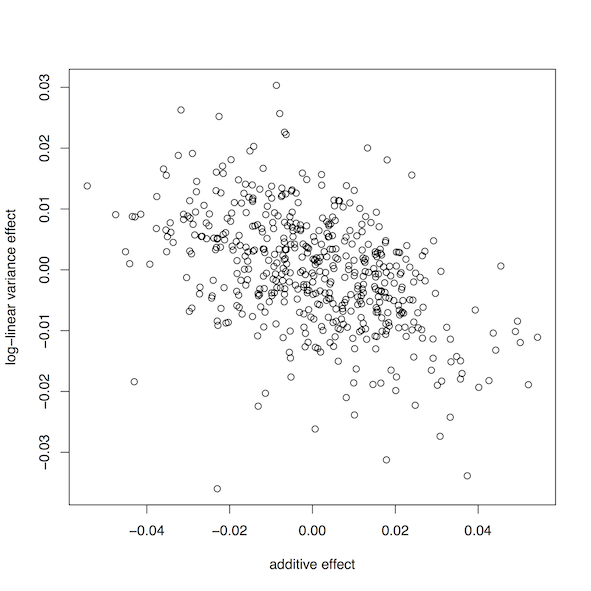
This shows a clear relationship between the additive effect of a SNP and its log-linear variance effect remains after inverse-normal transformation.

By inferring the relationship between additive effects and log-linear variance effects, one can estimate dispersion effects, which are effects on phenotypic variance that cannot be explained by a general mean-variance relation.

We have prepared an R script that estimates dispersion effects and adds them to the results table. To estimate dispersion effects, type

source('estimate_dispersion_effects.R')

The first SNP should have a dispersion effect. To see if there is evidence for this, example ‘results[1,]’, in particular, whether ‘dispersion_pval’ is large for the first SNP.

The other SNPs should not have dispersion effects. To test this, type

ks.test(results$dispersion_t[-1]^2,'pchisq',1)

The p-value should not be significant. This is in contrast to the log-linear variance effect p-value, which should be significant due to the general mean-variance relation.

We have shown how to infer additive, log-linear variance, and dispersion effects using HLMs (hetlm.model). We now show how to do the same while taking advantage of the favourable properties of linear mixed models for genetic association testing.

We model random effects for the genotypes in random.bed. All of these SNPs have (relatively weak) additive effects on the trait, so modelling random effects should increase power.

To fit HLMMs (hetlmm.model)to all loci in test.bed, at the UNIX terminal, type

python ../bin/hlmm_chr.py test.bed 0 500 test_phenotype.fam test_random --random_gts random.bed

This will output ‘test_random.models.gz’ with the results of fitting the heteroskedastic linear mixed model to the SNPs in test.bed

It is much more computationally demanding to fit the mixed model, so this may take some time depending on your computer. Alternatively, one can fit the models for the first 10 SNPs:

python ../bin/hlmm_chr.py test.bed 0 10 test_phenotype.fam test_random --random_gts random.bed

However, to estimate dispersion effects, one needs to have estimated additive and log-linear variance effects for a large number of SNPs. If one has fit models to all 500 SNPs, then one can analyse the results with the same process used for the non-mixed model analysis outlined above. The association signal for both additive and dispersion effects should be increased relative to the non-mixed model version.